Algorithms and Functions
Exercise 4.1. Two processes that you can use to multiply two nonnegative integers together are listed below:
Algorithm 4.1.
- Define a new number , and initialize it (i.e. set it equal) to 0.
- If , stop, and return the number .
- Otherwise, add to prod, and subtract 1 from . Then go to 2.
An example run of Algorithm 4.1 when :
Algorithm 4.2.
- Define a new number , and initialize it (i.e. set it equal) to 0.
- If , stop, and return the number .
- Otherwise, if is odd subtract from and set .
- Divide by 2, and multiply by 2.
- Go to step 2.
Similarly, an example run of Algorithm 4.2 when :
In general, which of these is the faster way to multiply two numbers? Why?
Functions in General
In your high-school mathematics classes, you’ve likely seen functions described as things like ” ” or ” .” When we’re writing code, however, we don’t do this! That is: in most programming languages, you can’t just type in expressions like the ones before and trust that the computer will understand what you mean. Instead, you’ll often write something like the following:
/* function returning the max between two numbers */
int max(int num1, int num2)
{
    /* local variable declaration */
    int result;

    if (num1 > num2)
        result = num1;
    else
        result = num2;

    return result;
}
Notice how in this example we didn’t just get to define the rules for our function: we also had to specify the kind of inputs the function should expect, and also the type of outputs the function will generate! On one hand, this creates more work for us at the start: we can’t just tell people our rules, and we’ll often find ourselves having to go back and edit our functions as we learn what sorts of inputs we actually want to generate.
On the other hand, though, this lets us describe a much broader class of functions than what we could do before! Under our old high-school definition for a function, we just assumed that functions took in numbers and returned numbers. With the above idea, though, we can have functions take in and output anything: multiple numbers, arrays, text files, whatever!
On the third(?) hand, enforcing certain restrictions on the types of inputs and outputs to a function is also a much more secure way to think about functions in computer science. If you’re writing code in a real-life situation, you should always expect malicious or just clueless users to try to input the worst possible data to your functions. As a result, you can’t just have a function defined by the rule and trust that your users out of the goodness of their hearts will never input 0 just to see what happens! They’ll do it immediately (as well as lots of other horrifying inputs, like 🐥, , ) just to see what happens.
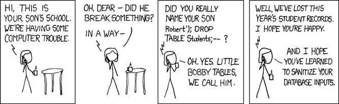
(from https://xkcd.com/327/)
This is why many programming languages enforce type systems: i.e. rules around their functions that specifically force you to declare the kinds of inputs and outputs ahead of time, like we’ve done above! Doing this is an important part of writing bug-free and secure code.
As this is a computer science class, we should have a definition of function that matches this concept. We provide this here:
- A collection of possible inputs. We call this the domain of our function.
- A collection describing the type of outputs that our function will generate. We call this the codomain of our function.
- A rule that takes in inputs from and generates outputs in .
Furthermore, in order for this all to be a function, we need it to satisfy the following property:
For every potential input from , there should be exactly one in such that . |
In other words, we never have a value in for which is undefined,as that would cause our programs to crash! As well, we also do not allow for a value to generate “multiple” outputs; i.e. we want to be able to rely on not changing on us without warning, if we keep the same.
Example 4.1. Typically, to define a function we’ll write something like “Consider the function , defined by the rule . This definition tells you three things: what the domain is (the set the arrow starts from, which is the integers in this case), what the codomain is (the set the arrow points to, which is the rational numbers in this case), and the rule used to define .
Example 4.2. defined by the rule ” if and only if ” is not a function. There are many reasons for this:
-
There are values in the domain that do not get mapped to any values in the codomain by our rule. For instance, consider . There is no value such that , because no integer when squared is negative! Therefore, is not mapped to any value in the codomain, and so we do not regard as a function.
-
There are also values in the domain that get mapped to multiple values in the codomain by our rule. For instance, consider . Because has the two solutions , this rule maps to the two values . This is another reason why is not a function!
Example 4.3. Let be the set of all students at the University of Auckland, and be the set of all integers. We can define a function by defining to be equal to that student’s current ID number. This is a function, because each student has a unique ID number!
However, if we tried to define a function by the rule the student whose ID number is , we would fail! This is because there are many integers that are not ID numbers: for example, no student has ID number , or .
While the objects above have had relatively “nice” rules, not all functions can be described quite so cleanly! Consider the following example:
Let be the collection {🇨🇦, 🐈, 🐥, 🇳🇿, 🕸️} of the Canada, cat, bird, New Zealand and web emojis, and let be the collection {🐙, ☢️, 🐝, 👨🏾} of the octopus, radiation, bee, and man emojis. Consider defined by the rules:
This is a function, because we have given an output for every possible input, and also never sends an input to multiple different outputs. It’s not a function with a simple algebraic rule like ” ”, but that’s OK!
A useful way to visualize functions defined in this piece-by-piece fashion is with a diagram: draw the domain at left, the codomain at right, and draw an arrow from each in the domain to its corresponding element in the codomain.
Alongside the domain/codomain ideas above, another useful idea here is the concept of range:
Note that the range is usually different to the codomain! In the examples we studied earlier, we saw the following:
- defined by the rule does not output every rational number! Amongst other values, it will never output any number greater than 1 (as for every integer .) As such, its codomain ( ) is not equal to its range.
- The function from Example 4.3, that takes in any student at the University of Auckland and outputs their student ID, does not output every integer: amongst other values, it will never output a negative integer! As such, its codomain ( ) is not equal to its range.
- The emoji function in Example 4.4 never outputs ☢️, even though it’s in the codomain.
Intuitively: we think of the codomain as letting us know what type of outputs we should expect. That is: in both mathematics or computer science, often just knowing that the output is “an integer” or “a binary string of length at most 20” or “a Unicode character” is enough for our compiler to work. As such, it’s often much faster to just describe the type of possible outputs, instead of laboriously finding out exactly what outputs are possible!
However, in some cases we will want to know precisely what values we get as outputs, and in that situation we will want to find the actual outputs: i.e. the range. To illustrate this, let’s consider a few examples:
Example 4.5. Consider the function given by the rule . This function has range equal to all even numbers that are at least 2.
To see why, simply notice that for any integer , is the “absolute value” of : i.e. it’s if we remove its sign so that it’s always nonnegative. As a result, is always a nonnegative even number, and this must be a nonnegative even number that’s at least 2.
That tells us that the only possible outputs are even numbers that are at least 2! However, we still don’t know that all of those outputs are ones that we actually can get as outputs.
To see why this is true: take any even number that is at least 2. By definition, we can write this as , for some . Rewrite this as ; if we do so, then we can see that (because if then and so .) As a result, we’ve shown that for any , and thus that we can actually get any even number that’s at least 2 as an output.
Example 4.6. Consider the emoji function from Example 4.4. If we look at the diagram we drew before, we can see that our function generates three possible outputs: 🐙, 🐝 and 👨🏾. Therefore, the collection of these three emojis is our range! | Domain 🇨🇦 🐥 🐈 🇳🇿 🕸️ Codomain 🐙 ☢️ 🐝 👨🏾 |
Example 4.7. Let be the collection of all pairs of words in the English language, and be the two values true, false . Define the function by saying that true if the words rhyme, and false otherwise. For example, cat, bat true, while cat, cataclysm is false.
The range of this function is true, false , i.e. the same as its codomain! It is possible for the range and codomain to agree. (If this happens, we call such a function a surjective function. We’re not going to focus on these functions here, but you’ll see more about them in courses like Compsci 225 and Maths 120/130!)
Example 4.8. Let denote the set of all real numbers (i.e. all numbers regardless of whether they’re rational or irrational; alternately, anything you can describe with a decimal expansion.) Define the function by the rule . This function has range equal to the set of all positive numbers! This takes more math to see than we currently have: again, take things like Maths 130 to see the “why” behind this. However, if you draw a graph of you’ll see that the outputs (i.e. -values) range over all of the possible positive numbers, as claimed. |  |
To close this section, we give a useful bit of notation for talking about functions defined in terms of other functions: function composition.
Fact 4.2. Given any two functions , we can combine these functions via function composition: that is, we can define the function , defined by the rule . We pronounce the small open circle symbol as “composed with.”
Example 4.9.
-
If are defined by the rules and then we would have .
-
Notice that this is different to !
In general, and are usually different functions: make sure to be careful with the order in which you compose functions.
-
If are defined by the rules and , then .
-
If and are defined by the rules and , then .
(Here, denotes the set of all positive real numbers.)
Handy!
Notice that in the definition above, we required that the domain of was the codomain of . That is: if we wanted to study , we needed to ensure that every output of is a valid input to .
This makes sense! If you tried to compose functions whose domains and codomains did not match up in this fashion, you’d get nonsense / crashes when the inner function returns an output at which the outer function is undefined. For example:
Example 4.10.
-
If is defined by the rule and is defined by the rule , then you might think that .
However, this is not a function! When , for example, we have , which is undefined. This is why we insist that the codomain of is the domain of ; we need all of ’s outputs to be valid inputs to .
-
Let be the set of all people in your tutorial room, be the set of all ID numbers of UoA students, and be the set of all ID numbers of Compsci 120 students. Then defined by taking any Compsci 120 student’s ID and outputting their grade on the mid-sem test is a function; as well, , defined by mapping each person in your tutorial room to their ID number is a function.
However, , the function that tries to take each person in your tutorial room and output their mid-sem test score, is undefined! In particular, your tutor is someone in your tutorial room, who even though they do have an ID number, will not have a score on the mid-sem test. Another reason to insist that the codomain of is the domain of !
Algorithms
In the previous section, we came up with a “general” concept for function that we claimed would be better for our needs in computer science, as it would let us think of things like
/* function returning the max between two numbers */
int max(int num1, int num2)
{
    /* local variable declaration */
    int result;

    if (num1 > num2)
        result = num1;
    else
        result = num2;

    return result;
}
as a function. However, most of the examples we studied in this chapter didn’t feel too much like the code above: they were either fairly mathematical in nature (i.e. ) or word-problem-oriented (i.e. the function that sent UoA students to their ID numbers.)
To fix this issue, this section will focus on the idea of an algorithm: that is, a way of describing in general a step-by-step problem-solving process that we can easily turn into code.
We start by describing what an algorithm is:
Typically, people think of algorithms as a set of instructions for solving some problem; when they do so, they typically have some restrictions in mind for the kinds of instructions they consider to be valid. For example, consider the following algorithm for proving the Riemann hypothesis:
- Prove the Riemann hypothesis.
- Rejoice!
On one hand, this is a fairly precise and unambiguous set of instructions: step 1 has us come up with a proof of the Riemann hypothesis, and step 2 tells us to rejoice.
On the other hand: this is not a terribly useful algorithm. In particular, its steps are in some sense “too big” to be of any use: they reduce the problem of proving the Riemann hypothesis to … proving the Riemann hypothesis. Typically, we’ll want to limit the steps in our algorithms to simple, mechanically-reproducible steps: i.e. operations that a computer could easily perform, or operations that a person could do with relatively minimal training.
In practice, the definition of “simple” depends on the context in which you are creating your algorithm. Consider the algorithm for making delicious pancakes, given at below.
An algorithm for pancakes!
- Acquire and measure out the following ingredients:
- 2 cups of buttermilk, or 1.5 cups milk + .5 cups yoghurt whisked together.
- 2 cups of flour.
- 2 tablespoons of sugar.
- 2 teaspoons of baking powder.
- 1/2 teaspoon of baking soda.
- 1/2 teaspoon of salt.
- 1 large egg.
- 3 tablespoons butter.
- Additional butter.
- Maple syrup.
- Whisk the flour, sugar, baking powder, baking soda, and salt in a medium bowl.
- Melt the 3 tablespoons of butter.
- Whisk the egg and melted butter into the milk until combined.
- Pour the milk mixture into the dry ingredients, and whisk until just combined (a few lumps should remain.)
- Heat a nonstick griddle/frypan on medium heat until hot; grease with a teaspoon or two of butter.
- Pour cup of batter onto the skillet. Repeat in various disjoint places until there is no spare room on the skillet. Leave gaps of 1cm between pancakes.
- Cook until large bubbles form and the edges set (i.e.\ turn a slightly darker color and are no longer liquid,) about 2 minutes.
- Using a spatula, flip pancakes, and cook a little less than 2 minutes longer, until golden brown.
- If there is still unused batter, go to 5; else, top pancakes with maple syrup and butter, and eat.
This is a good recipe. Use it!
This algorithm’s notion of “simple” is someone who is (1) able to measure out quantities of various foods, and (2) knows the meaning of various culinary operations like “whisk” and “flip.” If we wanted, we could make an algorithm that includes additional steps that define “whisking” and “flipping”. That is: at each step where we told someone to whisk the flour, we could instead have given them the following set of instructions:
(a). Grab a whisk. If you do not know what a whisk is, go to this Wikipedia article and grab the closest thing to a whisk that you can find. A fork will work if it is all that you can find. (b). Insert the whisk into the object you are whisking. (c). Move the whisk around through the object you are whisking in counterclockwise circles of varying diameter, in such a fashion to mix together the contents of the whisked object.
In this sense, we can extend our earlier algorithm to reflect a different notion of “simple,” where we no longer assume that our person knows how to whisk things. It still describes the same sets of steps, and in this sense is still the “same” algorithm — it just has more detail now!
This concept of “adding” or “removing” detail from an algorithm isn’t something that will always work; some algorithms will simply demand steps that cannot be implemented on some systems. For example, no matter how many times you type “sudo apt-get 2 cups of flour,” your laptop isn’t going to be able to implement our above pancake algorithm. As well, there may be times where a step that was previously considered “simple” becomes hideously complex on the system you’re trying to implement it on!
We’re not going to worry too much about the precise definition of “simple” in this class, because we’re not writing any code here (and so our notion of “simple” isn’t one we can precisely nail down) --- these are the details we’ll leave for your more coding-intensive courses.
Instead, let’s just look at a few examples of algorithms! We’ve already seen one in this class, when we defined the operation:
Algorithm 4.3. This algorithm takes in any two integers , where . It then calculates as follows:
- If , we repeatedly subtract from until , and return the end result.
- If , repeatedly add to until , and return the end result.
- If neither of these cases apply, then we just return .
Second, we can turn Claim 1.6 into an algorithm for how to tell if a number is prime:
Algorithm 4.4. This is an algorithm that takes in a positive integer , and determines whether or not is prime. It proceeds as follows:
- If , stop: is not prime.
- Otherwise, if , find all of the numbers . Take each of these numbers, and test whether they divide .
- If one of them does, then is not prime!
- Otherwise, if none of them divide , then by Claim 1.6, is prime.
This is a step-by-step process that tells us if a number is a prime or not! Notice that the algorithm itself didn’t need to contain a proof of Claim 1.6; it just has to give us instructions for how to complete a task, and not justify why those instructions will work. It is good form to provide such a justification where possible, as it will help others understand your code! However, it is worth noting that such a justification is separate from the algorithm itself: it is quite possible (and indeed, all too easy) to write something that works even though you don’t necessarily understand why.
For a third example, let’s consider an algorithm to sort a list:
Algorithm 4.5. The following algorithm, , takes in a list of numbers and orders it from least to greatest. For example, is . It does this by using the following algorithm:
- If contains at most one number, is trivially sorted! In this situation, stop.
- Otherwise, contains at least two numbers. Let , where . Define a pair of values , , and set them equal to the value and location of the first element in our list.
- One by one, starting with the second entry in our list and working our way through our entire list , compare the value stored in to the current value that we’re examining.
-
If , update to be equal to , and update to be equal to k.
-
Otherwise, just go on to the next value.
- At the end of this process, and describes the value and the location of the smallest element in our list. Swap the first value in our list with in our list: this makes the first value in our list the smallest element in our list.
- To finish, set the first element of our list aside and run on the rest of our list.
Back in our first chapter, to understand our two previous algorithms 4.3 and 4.4 we started by running these algorithms on a few example inputs! In general, this is a good tactic to use when studying algorithms; actually plugging in some concrete inputs can make othewise-obscure instructions much simpler to understand.
To do so here, let’s run our algorithm on the list , following each step as written:
Here, we use the , and boxes to visualize the “rest of our list” part of step 5 in our algorithm.
This worked! Moreover, doing this by hand can help us see an argument for why this algorithm works:
Proof. In general, there are three things we need to check to show that a given algorithm works:
-
The algorithm doesn’t have any bugs: i.e. every step of the process is defined, you don’t have any division by zero things or undefined cases, or stuff like that.
This is true here! The only steps we perform in this algorithm are comparisons and swaps, and the only case we encounter is ” is true” or ” is false,” which clearly covers all possible situations. As such, there are no undefined cases or undefined operations.
-
The algorithm doesn’t run forever: i.e. given a finite input, the algorithm will eventually stop and not enter an infinite loop.
This is also true here! To see why, let’s track the number of comparisons and write operations performed by this process, given a list of length as input:
-
Step 1: one comparisons (we checked the size of the list.)
-
Step 2: two write operations (we defined , .)
-
Step 3: comparisons and possibly write operations.
To see why: note that for all of the entries in our list from onwards, we looked up the value in and compared it to the value we have in , which gives us comparisons. If it was smaller, we rewrote the values in and in 3(a).
-
Step 4: 2 write operations (to swap these values.)
-
Step 5: 1 write operation (to resize the list to set the first element aside), and however many operations we need to sort a list of numbers with .
In total, then, we have the following formula: if denotes the maximum number of operations in total needed to sort a list with our algorithm, then
At first, this looks scary: our function is defined in terms of itself! In practice, though, this is fine. We know that , because step 1 immediately ends our program if the list has size 1.
Therefore, our formula above tells us that if we set , we have
by using our previously-determined value for . Still finite!
We can do this again for , and get
by using our previously-determined value for . Again, still finite!
In general, if this process can sort a list of size in finitely many steps, then it only takes us more steps to sort a list of size . In particular, there is no point at which our algorithm jumps to needing “infinitely many” steps to sort a list!
-
-
The algorithm produces the desired output: in this case, it produces a list ordered from least to greatest.
This happens! To see why, notice that in step 4, we always make the first element of the list we’re currently sorting the smallest element in our list. Therefore, on our first application of step 4, we have ensured that is the smallest element of our list.
On the second application of step 4, we were sorting the list starting from its second element: doing so ensures that is smaller than all of the remaining elements.
On the third application of step 4, we had set the first two elements aside and were sorting the list starting from its third element: doing so ensures that is smaller than all of the remaining elements.
In general, on the -th application of step 4, we had set the first elements aside and were sorting the list starting from its -th element! Again, doing so ensures that is smaller than all of the remaining elements.
So, in total, what does this mean? Well: by the above, we know that , as by definition each element is smaller than all of the ones that come afterwards. In other words, this list is sorted!
Recursion, Composition, and Algorithms
Algorithm 4.5 had an interesting element to its structure: in its fifth step, it contained a reference to itself! This sort of thing might feel like circular reasoning: how can you define an object in terms of itself?
However, if you think about it for a bit, this sort of thing is entirely natural: many tasks and processes in life consist of “self-referential” that are defined by self-reference! We call such definitions recursive definitions, and give a few examples here:
Example 4.11. Fractals, and the many plants and living things that have fractal-like patterns built into theirselves, are examples of recursively-defined objects! For example, consider the following recursive process:
- Start by drawing any shape . For example, here’s a very stylized drawing of a cluster of fern spores:

If you know some linear algebra, the explicit formulas we are using here are the following: for each point in , draw the four points
-
+ ,
-
,
-
,
-
,
This is the precise math-y way of describing the operations we’re doing to these rectangles!
-
Now, given any shape , we define as the shape made by making four copies of and manipulating them as follows: if is a shape contained within the gray rectangle at left, we make four copies of appropriately scaled/stretched/etc to match the four rectangles at right. (It can be hard to see the black rectangle, because it’s so squished: it’s the stem-looking bit at the bottom-middle.)

For example, , i.e. applied to our fern spore shape, is the following:

-
Using our “seed” shape and our function , we then recursively define as for every positive integer . That is: , etc. This is a recursive definition because we’re defining our shapes in terms of previous shapes! Using the language of function composition, we can express this all at once by writing .
-
Now, notice what these shapes look like as we draw several of them in a row:

Our seed grows into a fern!
This is not a biology class, and there are many open questions about precisely how plants use DNA to grow from a seed. However, the idea that many plants can be formed by taking a simple instruction (given one copy of a thing, split it into appropriately stretched/placed copies of that thing) and repeatedly applying it is one that should seem reasonable, given the number of places you see it in the world!
Example 4.12. On the less beautiful but more practical side, recursion is baked into many fundamental mathematical operations! For example, think about how you’d calculate . By definition, because multiplication is just repeated addition, you could calculate this as follows:
Now, however, suppose that someone asked you to calculate . While you could use the process above to find this product, you could also shortcut this process by noting that
This sort of trick is essentially recursion! That is: if you want, you could define the product recursively for any nonnegative integer by the following two-step process:
- , for every .
- For any , .
The second bullet point is a recursive definition, because we defined multiplication in terms of itself! In other words, when we say that , we’re really thinking of multiplication recursively: we’re not trying to calculate the whole thing out all at once, but instead are trying to just relate our problem to a previously-worked example.
Exponentiation does a similar thing! Because exponentiation is just repeated multiplication, we know that
Similarly, though, we can define exponentiation recursively by saying that for any nonnegative integer and nonzero number , that
- , and
- For any , .
In other words, with this idea, we can just say that
instead of calculating the entire thing from scratch!
These ideas can be useful if you’re working with code where you’re calculating a bunch of fairly similar products/exponents/etc. With recursion, you can store some precalculated values and just do a few extra steps of working rather than doing the whole thing out by scratch each time. Efficiency!
In classes like Compsci 220/320, you’ll study the idea of efficiency in depth, and come up with more sophisticated ideas than this one! In most practical real-life situations there are better ways to implement multiplication and exponentiation than this recursive idea; however, it can be useful in some places, and the general principle of “storing commonly-calculated values and extrapolating other values from those recursively” is one that does come up in lots of places!
Recursion also comes up in essentially every dynamical system that models the world around us! For instance, consider the following population modelling problem:
Example 4.13. Suppose that we have a petri dish in which we’re growing a population of amoebae, each of which can be in two possible states (small and large).
Amoebas grow as follows: if an amoeba is small at some time , then at time it becomes large, by eating food around it. If an amoeba is large at some time , then at time it splits into one large amoeba and one small amoeba.
Suppose our petri dish starts out with one small amoeba at time . How many amoebae in total will be in this dish at time , for any natural number ?
Answer. To help find an answer, let’s make a chart of our amoeba populations over the first six time steps:
This chart lets us make the following observations:
- The number of large amoebae at time is precisely the total number of amoebae at time . This is because every amoeba at time either grows into a large amoeba, or already was a large amoeba!
- The number of small amoebae at time is the number of large amoebae at time . This is because the only source of small amoebae are the large amoebae from the earlier step when they split!
- By combining 1 and 2 together, we can observe that the number of small amoebae at time is the total number of amoebae at time !
- Consequently, because we can count the total number of amoebae by adding the large amoebae to the small amoebae, we can conclude that the total number of amoebae at time is the total number of amoebae at time , plus the total number of amoebae at time . In symbols,
We call relations like the one above recurrence relations, and will study them in greater depth when we get to induction as a proof method.
For now, though, notice that they are remarkably useful objects! By generalizing the model above (i.e. subtracting to allow for old age killing off amoebas, or having a term to denote that as the population grows too large, predation or starvation will cause the population to die off, etc.) one can basically model an arbitrarily-complicated population over the long term.
These are particularly cool because they actually accurately model predator/prey relations in real life! See Isle Royale, amongst other examples. For more details on these sorts of population-modelling processes, see the logistic map, the Lotka-Volterra equations, and most of the applied mathematics major here at Auckland!
It bears noting that the amoeba recurrence relation is not the first recurrence relation you’ve seen! If you go back to Algorithm 4.5, we proved that
This is another recurrence relation: it describes the maximum number of operations needed to sort a list of size in terms of the maximum number of operations needed to sort a list of size .
While recurrence relations are nice, they can be a little annoying to work with directly. For example, suppose that someone asked us what is. Because we don’t have a non-recursive formula, the only thing we could do here is just keep recursively applying our formula, to get
= … |
This is … kinda tedious. It would be nice if we had a direct formula for this: something like or that we could just plug into and get an answer.
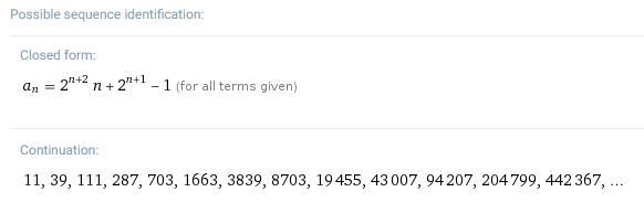
At this point in time, we don’t have enough mathematics to directly find such a “closed” form. However, we can still sometimes find an answer by just guessing. To be a bit more specific: if we use our definition, we can calculate the following values for :
To get these skills, either take Maths 120 and study linear algebra / eigenvalues, or take Compsci 220/320, or take Maths 326 and learn about generating functions!
If you plug this into the Online Encyclopedia of Integer Sequences, it will give you the following guess by comparing it to all of the sequences it knows:
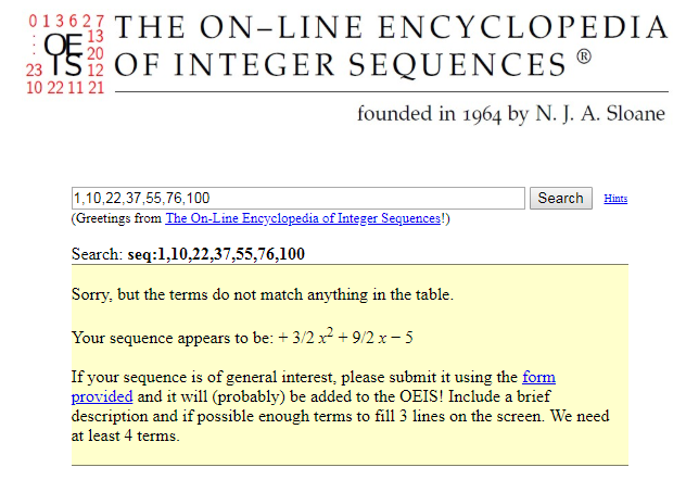
This turns out to be correct!
We don’t have the techniques to prove this just yet. If you would like to see a proof, though, skip ahead to the induction section of our proofs chapter! We’ll tackle this problem there (along with another recurrence relation), in Section 7.8.
Runtime and Algorithms
In the above few sections, we studied and analyzed the maximum number of operations it needs to sort a list of length . In general, this sort of run-time analysis of an algorithm - i.e. the number of elementary operations needed for that algorithm to run - is a very useful thing to be able to do!
To give a brief example of why this is useful, consider another, less well-known algorithm that we can use to sort a list:
Algorithm 4.6. The following algorithm, BogoSort , takes in a list of numbers and orders it from least to greatest. It does this by using the following algorithm:
-
One by one, starting with the first entry in our list and working our way through our list, compare the values stored in consecutive elements in our list.
If these elements never decrease - i.e. if when we perform these comparisons, we see that - then our list is already sorted! Stop.
-
Otherwise, our list is not already sorted. In this case, randomly shuffle the elements of our list around, and loop back to step 1.
Here’s a sample run of this algorithm on the list , where I’ve used Random.org to shuffle our list when needed by step 3:
This … is not great. If you used BogoSort to sort a deck of cards, your process would look like the following:
- One-by-one, go through your deck of cards and see if they’re ordered.
- If during this process you spot any cards that are out of order, throw the whole deck in the air, collect the cards together, and start again.
By studying the running time of this algorithm, we can make “not great” into something rigorous:
Proof. If is a list containing different elements, there are many different ways to order ’s elements (this is ordered choice without repetition, where we think of ordering our list as “choosing” elements one-by-one to put in order.) If all of these elements are different, then there is exactly one way for us to put these elements in order.
Therefore, on each iteration BogoSort has a chance of successfully sorting our list, and therefore has a chance of failing to sort our list. For any , is nonzero, and so the chance that our algorithm fails on any given iteration is nonzero.
Therefore, in the worst-case scenario, it is possible for our algorithm to just fail on each iteration, and thereby this algorithm could have infinite run-time.
In terms of running time, then, we’ve shown that BogoSort has a strictly worse runtime than , as . Success!
This sort of comparison was particularly easy to perform, as one of the two things we were comparing was . However, this comparison process can get trickier if we examine more interesting algorithms. Let’s consider a third sorting algorithm:
Algorithm 4.7. The following algorithm, MergeSort , takes in a list of numbers and orders it from least to greatest. It does this by using the following algorithm:
-
If contains at most one number, is trivially sorted! In this situation, stop.
-
Otherwise, contains at least two numbers. In this case,
(a) Split in half into two lists .
(b) Apply MergeSort to each of to sort them.
-
Now, we “merge” these two sorted lists:
(a) Create a big list with entries in it, all of which are initially blank.
(b)Compare the first element in to the first element in . If are both sorted, these first elements are the smallest elements in .
(c) Therefore, the smaller of those two first elements is the smallest element in our entire list. Take it, remove it from the list it came from, and put it in the first blank location in our big list.
(d) Repeat (b)+(c) until our big list is full!
As before, to better understand this algorithm, let’s run it on an example list like :
Here, we use the colored boxes to help us visualize the recursive applications of to smaller and smaller lists.
As before, it is worth taking a moment to explain why this algorithm works:
Proof. We proceed in the same way as when we studied :
-
Does the algorithm have any bugs? Nope! The only things we do in our algorithm are compare elements, split our lists, and copy elements over. Those are all well-defined things that can be done without dividing by zero or other sorts of disallowed operations!
-
Does the algorithm run forever? Nope!
To see why, let’s make a recurrence relation like we did before. To be precise:
Claim 4.5.Link copied If we let denote the maximum number of steps needed by MergeSort to sort a list of elements, then if is even. Proof. By definition, MergeSort performs the following operations:
- In step 1, it performs one operation (it looks up the size of the list.)
- In step 2, it splits the list in half. We can do this with at most write operations by just making two blank lists of size and copying elements over one-by-one to these new lists. It then runs MergeSort on each half. Doing this gives us an extra steps.
- In step 3, we repeatedly compare the first element in to the first element in , remove the smaller of the two elements from that list, and put it into our big list. This is one comparison and two write operations, which we did as many times as we had elements in our original list; so we have at most operations here in total.
In total, then, we have
If is odd, this gets a bit more annoying and we’d have (” rounded up”) plus (” rounded down”) here instead. This doesn’t materially change things, but it is annoying enough to warrant just looking at the even cases.
If we just round any odd-length list up to an even-length list by adding a blank cell, this gives us a recurrence relation that lets us reduce the task of calculating for any to the task of calculating smaller values of . Therefore this process cannot run forever, by the same reasoning as with !
-
Does the algorithm sort our list? Yes!
To see why, make the following observations:
-
Our algorithm trivially succeeds at sorting any list with one element.
-
Our algorithm also succeeds at sorting any list with 2 elements. To see why, note that by definition, it takes those two elements and splits them into two one-element lists. From there, it puts the smaller element from those two lists into the first position, and puts the larger in the second position, according to our rules. That’s a sorted list!
-
Now, consider any list on 3 or 4 elements. By definition, our algorithm will do the following:
- It takes that list, and splits it into two lists of size 1 or 2.
- It sorts those lists (and succeeds, by our statements above!)
- It then repeatedly takes the smaller of the first elements in either of those two lists, removes it from that list, and puts it into our larger list. Because those small lists are sorted, each time we do this we’re removing the smallest unsorted element (as the first element in a sorted list is its smallest element.) Therefore, this process puts elements into our largest list in order by size, and thus generates a sorted list.
So our process works on lists of 3 or 4 elements!
-
The same logic will tell us that our process works for lists on 5-8 elements: because any list on 5-8 elements will split into two lists of size at most 4, and our process works on lists of size at most 4, it will continue to succeed!
-
In general, our process will always work! This is because our process works by splitting in half, and thus it reduces the task of sorting a list of size into the task of sorting two lists of size . Repeatedly performing this reduction eventually reduces our task to just sorting a bunch of small lists, which we’ve shown here that we can do.
-
As well, by using the same sort of “guess-a-pattern” idea from before, we can refine this to a closed-form solution!
Note that if we use our definition, we can calculate the following values for . By definition, , as this algorithm stops when given any list of length 1. Therefore, by repeatedly using Claim 4.5, we can get the following:
which in table form is the following:
(Note that we’re using as the length of our lists. This is because our result only works for even numbers, so we want something that stays even when we keep dividing it by 2.)
Spotting the pattern here is a pain without more advanced mathematics; even the Online Encyclopedia of Integer Sequences doesn’t recognize it. WolframAlpha, however, does!
Again, this is a claim whose proof will have to wait for Section 7.8. For now, though, let’s take the following as given:
We can easily extend this to a list whose length is not a power of two by just “rounding its length up to the nearest power of 2” by adding in some blank cells: i.e. if we had a list of length 28, we’d add in 4 blank cells to get a list of length 32.
If we do this, then Claim 4.6 becomes the following:
To simplify this a bit to just write things in terms of , notice that if is rounded up to the nearest power of 2, then Plug this into Observation 4.10, and you’ll get the following:
Recall that is ” rounded up.”
Two useful tricks we’re using in this calculation:
- . That is: rounding a number up only makes it larger.
- . That is: rounding up never increases a number by more than 1.
Nice! This is worth making into its own observation:
Comparing Runtimes: Limits
Now, we have an interesting problem on our hands: between and , which of these two algorithms is the most efficient?
That is: in terms of functions, which of the following is better?
vs.
To start, we can make a table to compare values:
It looks like the algorithm needs more steps than so far. However, this table only calculated the first few values of ; in real life, however, we often find ourselves sorting huge lists! So: in the long run, which should we prefer?
To answer this, we need the idea of a limit:
If you would like a more rigorous definition here than “gets close”, look into classes like Maths 130 and Maths 250!
This is a tricky concept! To understand it, let’s look at a handful of examples:
Problem 4.1. What is ?
Answer. First, notice that as goes to infinity, goes to 0, because its denominator is going to infinity while the numerator stays fixed.
Therefore, goes to 2, and so
Problem 4.2. What is ?
Answer. . This is because for any positive integer , we can make by setting to be any value .
In other words, as grows, it eventually gets larger than for any fixed , and thus itself grows without bound.
Problem 4.3. What is ?
Answer. To find this limit, we simply break our function down into smaller pieces:
- First, notice that as takes on increasingly large positive values, goes to 0 and stays positive.
- Therefore, goes to negative infinity, as tiny positive numbers yields increasingly huge negative numbers.
- Therefore, goes to 0, as yields tiny negative numbers.
In total, then,
Problem 4.4. What is ?
Answer. It is tempting to just “plug in infinity” into the fraction above, and say that
“because our limit is 1”
However, you can’t do manipulations like this with infinity! For example, because , we have
even though the method above would say that
“because our limit is 1.”
The issue here is that there are different growth rates at which various expressions approach infinity: i.e. in our example above, approaches infinity considerably faster than , and so the ratio approaches 0 even though the numerator and denominator individually approach infinity.
Instead, if we ever have both the numerator and denominator approaching , we need to first simplify our fraction to proceed further! In this problem, notice that if we divide both the numerator and the denominator by the highest power present in either the numerator or denominator, we get the following:
As noted above, each of go to 0 as goes to infinity, because their denominators are going off to infinity while the numerator is staying fixed.
Therefore, we have
With the idea of limits in mind, we can now talk about how to compare functions:
Intuitively, this definition is saying that for huge values of , the ratio of to goes to infinity: that is, is eventually as many times larger than as we could want.
We work an example of this idea here, to see how it works in practice:
Example 4.14. We claim that the function grows faster than . To see this, by our definition above, we want to look at the limit .
Notice that we can factor the numerator into . Plugging this into our fraction leaves us with , which we can simplify (as in Problem 4.4.) to .
As goes to infinity, goes to infinity.
This grows without bound: as goes to infinity, so does ! Therefore we’ve shown that grows faster than .
To deal with a comparison like the one we’re trying to do between and , however, we need some more tricks!
Limit Techniques and Heuristics
Without calculus, our techniques for limits are a little hamstrung. As those of you who have seen NCEA L3 calculus, things like L’H^opital’s rule are extremely useful for quickly evaluating limits!
With that said, though, we do have a handful of useful techniques and heuristics that we can use to get by. Here’s an easy (if not very rigorous) technique:
For instance, suppose that we wanted to compare the runtime of our two functions and . By definition, this means that we want to find the limit
To do this, we could just plug in various values of and see what happens!
It certainly looks like is growing arbitrarily large, so we could quite reasonably believe that the number of steps required to calculate is growing faster than the number of steps needed to calculate (and thus is the preferable algorithm.)
However, this method has its limitations:
-
One issue with the above is that it is fairly prone to human error if you’re manually doing this by plugging numbers into a calculator. That is: if you have a limit like , and you’re trying to plug in something like into that fraction, it’s going to be really easy to forget a zero in one of those expressions.
-
Another is that it can be pretty hard to tell whether or not you’re actually plugging in enough values to figure out the pattern! For example, when we made our table to compare the runtimes of these two functions by listing values from 1 through 7, we thought that was growing faster. This larger table seems to be telling the opposite story: but maybe the situation will reverse itself again if we zoom out further!
To give a second example, suppose that someone asked you to calculate
If you plugged in , you’d get . This looks like it’s slowly increasing to 0, so you’d be tempted to guess that
This is very false! As we saw before, as goes to infinity, goes to infinity. Therefore, also goes to infinity, and in general any composition of logs will eventually go off to infinity as well: i.e. is the correct limit here. So plugging things in can lead us to make mistakes!
A second technique, that we used in several of our worked problems earlier, is the following:
This often gives you a new function where you no longer have the top and bottom going to zero, which is often much easier to work with.
Example 4.15. If we had the limit , we could factor an out of the top and bottom to get . This is .
For a second example, if we had the limit , we could factor an out of the top and bottom to get the simplified limit . The numerator goes to 1 and the denominator just is 1, so this is 1.
Sometimes, however, we don’t have something that we can easily express as a fraction:
Problem 4.5. What is the limit
To approach this limit, we need another technique:
To understand this method, let’s apply it to Problem 4.5.
Answer to Problem 4.5. Understanding the function in our limit all at once is hard! But, notice that for very large values of , we know that
- is a very small positive number, therefore
- is basically , which is slightly larger than 1, therefore
- is basically slightly larger than 1 , and so in turn is a tiny negative number, therefore
- is 1 over a tiny negative number, and thus is an increasingly huge negative number.
Therefore, as goes to positive infinity goes to , and we’ve found our limit by breaking our function down into smaller pieces!
where ” ” means “grows slower than.”
Within those groups, we sort these expressions by degrees and bases: i.e.
and
and so on / so forth.
Finally, any sum of expressions grows as fast as its largest expression: i.e. a factorial plus a log plus a constant grows at a factorial rate, a plus a log plus a square root grows as fast as grows, etc.
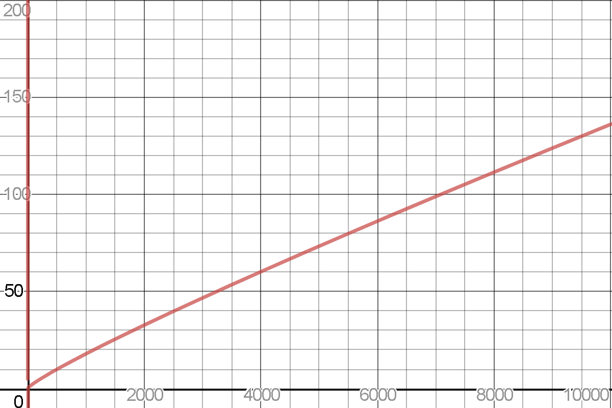
As a brief justification for this, let’s look at a table:
Above, we’ve plotted five algorithms with runtimes versus input sizes for ranging from to , with the assumption that we can perform one step every seconds.
In this table, you can make the following observations:
- The constant-runtime algorithm is great!
- The logarithmic-runtime algorithm is also pretty great!
- The polynomial-runtime algorithms all take longer than the constant or log algorithm, but are all at least reasonable.
- The exponential runtime algorithm starts off OK, but gets horrible fast\ldots
- … but is somehow not as bad as the factorial-runtime algorithm, which is almost immediately unusable for any value of .
We can use this heuristic to quickly answer our question about which of and is preferable, without having to plug in any numbers at all!
Proof. As noted before, by definition, we want to find the limit
By dividing through both sides by , this means that we’re looking at the ratio
The top is a linear expression (i.e. polynomial of degree 1), as the largest-growing object in the numerator is the term. The bottom, conversely, is a logarithmic expression, as the fastest-growing object in the denominator is the term.
Linear expressions grow much faster than logs, so our “plug things in” step didn’t lie: is growing faster than (and thus is the preferable algorithm, as in the long run it will need to perform less operations to get to the same answer.)
To study one more example of this idea and finish our chapter, let’s use this principle to answer our last exercise:
Answer to 4.1. In this problem, we had two multiplication algorithms and wanted to determine which is best.
Algorithm 4.1. calculated by basically just calculating . As such, its runtime is pretty much just some constant times ; we need iterations of this process to calculate the answer here, and we can let our constant be the number of steps we perform in each iteration.
Conversely, Algorithm 4.2. ran by taking and repeatedly subtracting 1 from and dividing by 2 until it was 0 (while doing some other stuff.)
For the purpose of this problem, we don’t have to think about why this process works, though look at practice problem 6 if you’re curious! Instead, if we simply take it on faith that this algorithm does work, it’s easy to calculate how long it takes to complete: it will need as many iterations as it takes to reduce to 0 by these operations.
In the worst-case scenario for the number of iterations, we only ever divide by 2; i.e. is a power of 2. In this case, it takes iterations if ; i.e. we need iterations, and thus need a constant times many operations.
As we saw before, logarithms grow much slower than linear functions! Therefore, Algorithm 4.2. is likely the better algorithm to work with.
Practice Problems
-
(-) Your two friends, Jiawei and Francis, have written a pair of algorithms to solve a problem. On an input of size , Jiawei’s algorithm needs to perform calculations to find the answer, while Francis’s algorithm needs to perform calculations to find the same answer.
Jiawei says that their algorithm is faster, because their runtime is polynomial while Francis’s algorithm has an exponential in it. Francis says that their algorithm is faster, because their algorithm has a logarithm in it while Jiawei’s is polynomial.
Who is right, and why?
-
(-) Let and . Calculate the following compositions:
-
We say that a function has an inverse if there is some function such that for all : that is, “undoes” , and vice-versa. For example, and are inverses, as is and .
- Suppose that . Find ’s inverse.
- Now, suppose that . Does this constant function have an inverse?
-
Let be the collection of all students enrolled at the University of Auckland and be the collection of classes currently running at the University of Auckland. Which of the following are functions?
- The rule , that given any student outputs the classes they’re enrolled in.
- The rule , that given any class outputs the student with the top mark in that class.
- The rule , that given any student outputs that student.
- The rule , that given any class outputs its prerequisites.
-
You’re a programmer! You’ve found yourself dealing with a program that has no comments in its code, and you want to know what it does. After some experimentation, you’ve found that takes in as input an integer , and does the following:
(i) Take and square it. (ii) If is 1, 2, 3 or 6, output and stop. (iii) Otherwise, replace with , i.e. the last digit of , and go to (ii) |
- Is a function, if we think of its domain and codomain as ?
- What is the range of ?
-
(+) Show that after each step in Algorithm 4.2., the quantity is always the same. Using this, prove that Algorithm 4.2. works!
-
(+) In our answer to 4.1., we used a sort of handwave-y “this takes about many operations” argument. Let’s make this more rigorous!
That is: let denote the number of steps that this algorithm needs to multiply a given number by .
- Find a recurrence relation in terms of , that holds whenever is even.
- Use this relation to calculate for , and plug these values into either the Online Encyclopedia of Integer Sequences or WolframAlpha. What pattern do you see?
-
Consider the following sorting algorithm, called :
Algorithm 4.8. The following algorithm, , takes in a list of numbers and orders it from least to greatest. It does this by using the following algorithm:
(i) Compare to . If , swap these two values; otherwise, leave them where they are.
(ii) Now, move on, and compare the “next” pair of adjacent values . Again, if these elements are out of order (i.e. ) swap them.
(iii) Keep doing this through the entire list!
(iv) At the end of this process, if you made no swaps, stop: your list is in order, by definition. Stop!
(v) Otherwise, the list might be out of order! Return to (i).
(a) Use this process to sort the list .
(b) (+) Let denote the maximum number of steps that needs to sort a list of length . Find an expression for , and calculate its values for and .
(c) What is the smallest number of steps that would need to sort a list of length ?
-
Find the following limits:
- Which of the three algorithms , and is the fastest (i.e. needs the fewest operations) to sort a list of 5 elements? Which needs the fewest to sort a list of 10 elements? How about 100? How about for huge values of ?