Graphs

Exercise 5.1. In the 1700’s, the city of Königsberg was divided by the river Pregel into four parts: a northern region, a southern region, and two islands. These regions were connected by seven bridges, drawn in red in the map below.

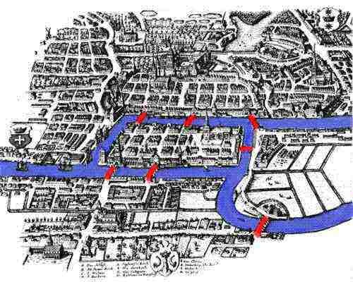
(A map of Königsberg, c. 1730. Source: Wikipedia)

These bridges were particularly beautiful pieces of architecture, and so when people would offer tours of the city they would try to take tourists across each bridge to show it off. However, tour guides at the time noticed that no matter how they could construct their walks around the city, they’d always either miss a bridge or have to double a few bridges up: they could never find a “perfect” tour that crossed each bridge exactly once.

Can you find such a tour? That is: can you come up with a walk through the city that starts and ends at the same place, and walks over each bridge exactly once?

Exercise 5.2. You’re a civil engineer! Suppose that you have a set of buildings, and you want to hook up each of these buildings to the city’s utilities, namely water, gas, and electricity.

However, your city is very earthquake-prone. As a safety precaution, they’ve asked that no two utilities are allowed to vertically “cross over” each other: that is, you can’t have water mains running beneath the gas mains, or gas pipes running above the electricity wires. So, for example, while the configuration drawn below wouldn’t work for two buildings, the right one would!

Can you connect three buildings to your utilities? Or is this impossible?__

Graph Theory

The field of graph theory originally started as a branch of “recreational mathematics,” and specifically as the puzzle in Exercise 5.1. Until the 1900’s, people viewed graph theory as a branch of mathematics used to solve riddles similar to the Konigsburg bridge problem, such as the following:

• Can you take a dodecahedron, start from one corner, and walk along the edges in a way that visits every other vertex exactly once and returns to where you start?

(A solution to the dodecahedron puzzle! Source: Wikipedia)

• Take a knight, and put it in the top-right-hand corner of an $8 \times 8$ chessboard. Can you move it around so that it visits every other square on the board exactly once, and returns to where it started?

• Take a box, divided into five rectangles. Can you draw a single continuous line that crosses each wall exactly once?

In recent years, however, mathematicians and computer scientists have transformed graph theory into one of the most applicable fields of mathematics in existence. Its power to describe networks has made it the perfect tool for studying many problems in the modern world; graphs can be used to model the internet, social networks, the spread of diseases through a population, travel, computer chip design, and countless other phenomena. Graphs are everywhere in the modern world, and their analysis is key to solving many of the most important problems of the 21st century.

In these notes, we’ll start by building up some definitions that will let us talk about graphs and their properties; from there, we’ll describe how to model various real-life objects with graphs, and then transition to solving a few real-life problems with graphs. This is (as with everything in this class) just the tip of the iceberg; if you want to see more, take papers like Compsci 225 and Maths 326!

We start with an intuitive definition of a graph:

Example 5.1. For example, all of the following objects can be thought of as graphs:

• Consider Facebook, or any other social network. You can think of any of these objects as consisting of two things: (1) the people, and (2) the connections (i.e. friendship, or following) between people.
• Think about the internet. You can model this as a collection of webpages, connected by links.
• Alternately, you can model the internet as a collection of computers, connected by cables/wireless signals.
• Look at all of New Zealand! You can model the country as a collection of cities, connected by roads.
• Alternately, you can choose to model New Zealand as a collection of regions, with two regions linked up if there’s a direct flight from one to the other.

If Definition 5.1 above feels a bit too informal for you, here’s a more precise way to describe a graph:

Example 5.2. The following describes a graph $G$ :

• $V = \{a,b,c,d,e\}$
• $E = \{ {\scriptstyle\{a,b\}}, {\scriptstyle\{b,c\}}, {\scriptstyle\{c,d\}} , {\scriptstyle\{d,e\}}, {\scriptstyle\{e,a\}} \}$

Given a graph $G = (V,E)$ , we can visualize $G$ by drawing its vertices as points on a piece of paper, and its edges as connections between those points.

Several ways of drawing the graph $G$ defined above are drawn at right. Notice that there are many ways to draw the same graph! Also note that edges don’t have to be straight lines, and that we allow them to cross.

In general, it is often much easier to describe a graph by drawing it rather than listing its vertices and edges one-by-one. Wherever we can, we’ll describe graphs by drawing pictures; we encourage you to do the same!

Here’s a few examples of graphs, described with this vertex+edge language:

Example 5.3.

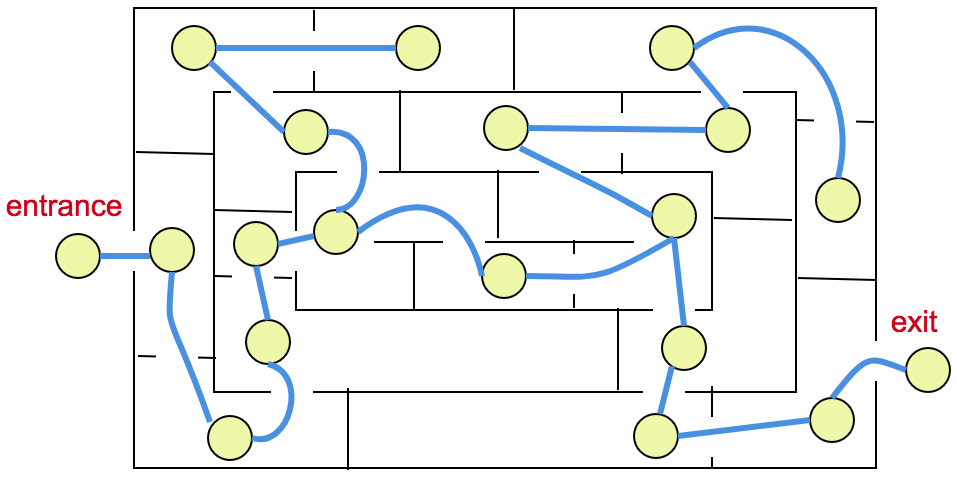
• We can represent a maze as a graph! Take the collection of “rooms” in our maze, and think of them as our vertices. Now, connect any two room-vertices with an edge if they are linked by a doorway.

  

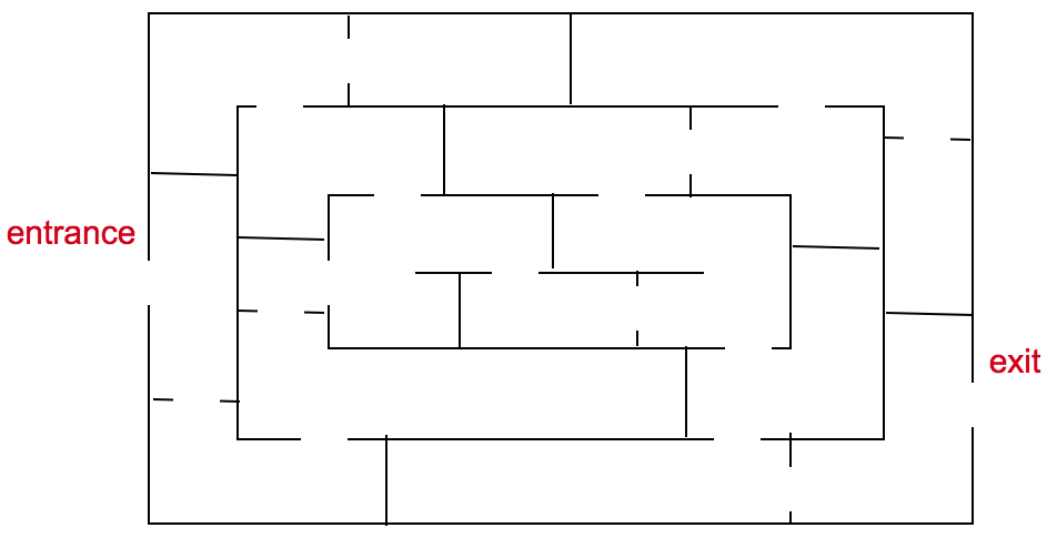
  With this done, finding a way out of our maze is the same as finding a walk through our graph! This can often simplify things for us, as the graph visualization lets us ignore some of the more irrelevant information (i.e. right angles, walls without doors, etc) in the maze.

  

• You and your three flatmates (Aang, Korra, and Zuko) have just moved to a new house. You have a list of tasks to do over the weekend: you all want to paint the walls, move in your furniture, cook dinner, and do some gardening. Suppose that you have the following skills:

  • You really like to paint and garden.
  • Aang is a great cook who enjoys gardening.
  • Zuko is also a great cook who’s strong (furniture.)
  • Korra is strong (furniture) and likes to paint.

You can visualize this with a graph! Make a vertex for each flatmate, and a vertex for each task. Then, connect flatmates to their preferred tasks with edges. With this, a “good” way to divide up tasks is to find a “matching:” that is, a way to pick out four edges in our graph, such that every person and every task is in exactly one edge (so that the work is divided!) Such a matching is highlighted in the graph at right.

Just as there are many different ways to model the connections between a set of objects, there are other notions of graphs beyond that of a simple graph. Here are some such definitions:

Definition 5.3.Link copied A simple graph with loops is just like a simple graph $G$ , except we no longer require the pairs of elements in $E$ to be distinct; that is, we can have things like $\{v,v\} \in E$ . A multigraph is a simple graph, except we allow ourselves to repeat edges in $E$ multiple times; i.e. we could have three distinct edges $e_1, e_2, e_3 \in E$ with each equal to the same pair $\{x,y\}$ . A directed graph is a simple graph, except we think of our edges as ordered pairs: i.e. we have things like $x \to y \in E$ , not $\{x,y\}$

You can mix-and-match these definitions: you can have a directed graph with loops, or a multigraph with loops but not directions, or pretty much anything else you’d want!

Remark 5.1. In this course, we’ll assume that the word graph means simple undirected graph without loops unless explicitly stated otherwise.

There are a handful of graphs that come up frequently in computer science and mathematics, are worth giving specific names. We describe a few of these graphs here:

Definition 5.4.Link copied The complete graph on $n$ vertices $K_n$ is defined for any positive integer $n$ as follows: take $n$ vertices. Now, take every possible pair of distinct vertices, and connect them with an edge! We draw several examples. In this sense, a complete graph is a graph in which we have as many edges as is possible for a graph on $n$ vertices.

To practice all of this graph theory language, let’s try solving one of our exercises!

Answer to Exercise 5.2. You cannot solve the utility problem!

To see why, let’s use the language of graph theory. Make each of our three buildings into vertices; as well, make each of the three utilities into vertices. If we connect each building to each utility, notice that we’ve created the graph $K_{3,3}!$

We claim that $K_{3,3}$ cannot be drawn without any edges crossing, and thus that this puzzle cannot be solved. To see why this is true, let’s use the “contradiction” technique we used above.

Think about what a solution would look like. In particular, notice that $K_{3,3}$ contains a “hexagon,” i.e. a $C_6$ , as drawn below. Therefore, in any drawing of $K_{3,3}$ , we will have to draw this cycle $C_6$ first.

Because this cycle is a closed loop, it separates space into an “inside” and an “outside.” Therefore, if we are drawing $K_{3,3}$ without edges crossing, after drawing the $C_6$ part, any remaining edge will have to either be drawn entirely “inside” the $C_6$ or “outside” the $C_6$ . That is, we can’t have an edge cross from inside to outside or vice-versa, because that would involve us crossing over pre-existing edges.

Therefore, if we have a crossing-free drawing of $K_{3,3}$ , after we draw the $C_6$ part of this graph, when we go to draw the $\{d,c\}$ edge we have two options: either draw this edge entirely on the inside of our $C_6$ , or entirely on the outside.

If we draw this edge on the inside, then on the inside the vertices $f$ and $a$ are separated by this edge; therefore, to draw the edge $\{a,f\}$ we must go around the outside. Similarly, if we draw this edge on the outside, then $a,f$ are separated from each other on any outside walk, and the edge $\{a,f\}$ must be drawn inside of the hexagon.

In either of these cases, notice that there is no walk that can be drawn from $b$ to $e$ on either the inside or the outside! Therefore we cannot draw our last edge $\{b,e\}$ without having a crossing, and thus have a contradiction to our claim that such a crossing-free drawing of $K_{3,3}$ was possible.

Graphs: Useful Concepts

In the above section, we saw how some of the language of graph theory could help us solve problems. In this section, we explore a number of other definitions and concepts that can come in handy!

Example 5.4. If we look at the flatmate graph from Example 5.3. above, we can see that the vertices “You” and “Paint” are adjacent, but that “You” and “Furniture” are not adjacent. Similarly, “Aang” and “Cook” are adjacent, but “Aang” and “Zuko” are not adjacent.

Notice that adjacency is just a property of individual edges! Even though we drew the Aang and Zuko vertices next to each other on our graph, we did not connect them with an edge, so they are not connected. As well, even though you can go from “You” to “Furniture” by using the multiple-edge walk

you cannot go from “You” to “Furniture” with a single edge, and so these vertices are not adjacent.

It is often useful to be able to refer to all of the neighbors of a vertex: in this graph, for instance, “Korra” is neighbors with “Paint” and “Furniture.”

Example 5.5. In the graph with red vertices drawn below, the vertex $a$ has degree 0, the vertex $b$ has degree 1, the vertices $d$ and $e$ have degree 2, and the vertex $c$ has degree 3.

Notice that a vertex can have degree 0: i.e. it is possible to have a vertex with no edges! This will often represent an “isolated” object in our graph: i.e. something without any connections to our wider graph.

Exercise 5.3. A bit more practice with the concept of degree: convince yourself of the following claims!

• The degree of every vertex in $K_n$ is $n-1.$
• The only possible degrees in $K_{m,n}$ are $m$ and $n.$
• The degree of every vertex in a cycle graph $C_n$ is 2.

To practice these concepts, let’s try writing a few arguments:

Proof. We can prove this by “counting” the number of times vertices in our graph show up as endpoints of edges in our graph. Notice that we could do this in two different ways:

• On one hand, every edge has two endpoints. Therefore, the total number of times vertices are used as endpoints in our graph is simply twice the number of edges.
• On the other hand, every endpoint is counted once when we calculate the degree of the corresponding vertex. Therefore, if we sum up the degrees of all of the vertices in our graph, this counts the total number of times vertices are used as endpoints in our graph.

However, both of these ways were counting the same thing! Therefore, we know that the answer we got from (1) must be the same as the answer we got in (2). In other words, the sum of degrees of vertices in our graph must be twice the number of edges, as claimed.

Example 5.6. In the graph at right, we have four vertices of degree 2, five vertices of degree 3, and one vertex of degree 5. Therefore, the sum of degrees in this graph is $4 \cdot 2 + 5 \cdot 3 + 1 \cdot 5 = 28$ .

Claim 5.1 says that this should be twice the number of edges; i.e. that this graph should have 14 edges. This is true: count them by hand!

This formula comes up often in graph theory, especially when trying to show that certain types of graphs are “impossible!” Consider the following result:

Proof. Before reading this proof, try to show this yourself: that is, take pen and paper, and try to draw a graph on seven vertices where all of the degrees are 3!

In doing so, we make two claims:

• You won’t succeed: you’ll always wind up with one vertex forced to have degree 2 or 4 (or you’ll accidentally make something that’s not a simple graph by drawing multiple edges / loops.)
• It won’t be obvious why this keeps failing: i.e. there will be a lot of different things you could have tried, and writing down a “proof” for why this is impossible may feel like it would involve a ton of tedious casework.

However, if we use the degree-sum formula, we claim that this problem is quite simple! We start by using a principle that’s served us well in many prior problems: let’s suppose that our claim is somehow false, and it is possible to have a graph $G$ on seven vertices in which all degrees are 3.

The degree-sum formula, when applied to $G$ , tells us that the sum of the degrees in $G$ must be twice the number of edges. Because all of the degrees in $G$ are 3 and there are seven vertices, we know that this degree sum is just $3 \cdot 7 = 21$ .

Therefore, we must have that two times the number of edges in our graph is 21. That is, we have $10.5$ edges \ldots which is impossible, because edges come in whole-number quantities! (I.e. you either have an edge $\{a,b\}$ or you don’t: there is no “half” of an edge $\fbox{\{a}$ in a simple graph.)

Therefore, such a graph $G$ cannot exist, as the number of edges required for such a graph $G$ is impossible to construct. In other words, no graphs exist on seven vertices in which all degrees are 3!

Walks and Connectedness

In several of the examples we looked at earlier, the idea of a walk through a graph was an incredibly useful one:

• In the “internet” graph, if we model this graph as a collection of computers connected by cables/wireless signals, in order for two people to communicate (i.e. send an email,) we have to find a way through this graph that links these two computers together.

• In the Konigsberg bridge problem from Example 5.1., we can turn the city of Konigsberg into a multigraph by making the four regions of the city into vertices, and connecting these vertices with edges.

In this setting, our goal is to find a walk through this graph that uses every edge exactly once, and starts + ends at the same place.

• In the “maze” graph, we wanted to find a walk through our graph that starts at the entrance and leaves through the exit.

• In the New Zealand graph, where we had a bunch of cities as our vertices connected by roads, we often want to navigate from one city to the next. Doing so is finding a route through our graph!

As such, we should come up with a definition for what a “walk” is in a graph:

We say that this walk starts at $v_0$ and ends at $v_n.$

We say that a walk is a circuit or closed walk if it starts where it ends; i.e. if $v_0 =v_n$ .

We say that a walk is a path if it does not repeat any vertices. A walk is a cycle if the first and last vertex of this walk are the same and all of the others are distinct.

We often describe a walk by just listing its vertices in order: i.e.

is a valid way to describe a walk.

Example 5.7. In the graph below, the following sequences are walks from $e$ to $g$ :

• $e \to a \to f \to b \to e \to d \to f \to b \to g$
• $e \to c \to g$

Notice that walks can repeat edges and vertices!

A useful property that graphs can have, related to this concept of walks, is being connected:

Example 5.8. The boxed graph below is not connected, as there is no path from $a$ to $b$ in this graph. The one at right, however, is connected, as there is a path from any vertex to any other vertex.

In many applications, we’ll want to find the shortest path between two objects: i.e. in a transit graph you’ll want to find the path with the shortest possible length, or in the internet graph you’ll want to find the path with the lowest total ping. To capture this idea, we’ll often want to attach weights to the edges of our graph, to represent paths that are physically longer / more expensive to use / etc. We do this as follows:

Example 5.9. A map of the South Island of New Zealand is drawn below. We can turn this into a graph by replacing each region with a vertex, and connecting two regions if they border each other.

With this done, we can turn this graph into a weighted graph by labelling each edge with the total amount of time it would take you to drive from the largest city in one region to the largest city in the next region. This gives us the graph below:

In graphs like this, we’ll often solve problems like the following:

Example 5.10. Suppose that you’re a traveling salesman. In particular, you’re traveling the South Island, and trying to sell rugby tickets for nine rugby teams there (one for each region in the map above.)

You want to start and finish in Mid-Canterbury, and visit each other region exactly once to sell tickets in it. What circuit can you take through these cities that minimizes your total travel time, while still visiting each city exactly once?

Without knowing any mathematics, you’d probably guess that the shortest route is to just go around the perimeter of the island. Intuitively, at the least, this makes sense: avoiding the southern alps is probably a good way to save time!

In real life, however, maps can get a lot messier than this. Consider a map of all of the airports in the world, or even just in New Zealand.

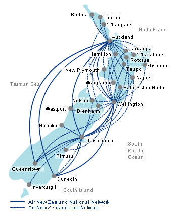
(Publicly-available Air New Zealand map sourced from Airline Route Maps)

If you were an Air New Zealand representative and wanted to visit each airport, how would you do so in the shortest amount of time and still return home to Auckland?

In general: suppose you have $n$ cities $C_1, \ldots C_n$ that you need to visit for work, and you’re trying to come up with an order to visit them in that’s the fastest. For each pair of cities $\{C_i, C_j\}$ , assume that you know the time it takes to travel from $C_i$ to $C_j$ . How can you find the cheapest way to visit each city exactly once, so that you start and end at the same place?

These sorts of tasks are known as traveling salesman problems, and companies all over the world solve them daily to move pilots, cargo, and people to where they need to be. Given that it’s a remarkably practical problem, you’d think that we’d have a good solution to this problem by now, right?

… not so much. Finding a “quick” solution (i.e. one with non-exponential runtime) to the traveling salesman problem is an open problem in theoretical computer science; if you could do this, you would solve a problem that’s stumped mathematicians for nearly a century, advance mathematics and computer science into a new golden age, and quite likely go down in history as one of the greatest minds of the millenium.

This is a fancy way of saying “this problem is really hard.” So: why mention it here? Well: in computer science in general, and graph theory in particular, we often find ourselves having to solve problems that don’t have known good or efficient algorithms. Despite this, people expect us to find answers anyways: so it’s useful to know how to find “good enough” solutions in cases like this!

For the traveling salesman problem, one brute-force approach you could use to find the answer could be coded like this:

Algorithm 5.9. Init: Take our graph $G$ , containing $n$ vertices. Let $s$ be the vertex we start and end at. Let $c$ be a cost function, that given any edge $\{x,y\}$ in $G$ outputs the cost of traveling along that edge.

• Write down every possible walk in which we can list the $n$ vertices of $G$ , starting and ending at $s$ .

• For each walk ${\{s,v_1\}}, {\{v_1,v_2\}},\ldots, {\{v_{n-1},v_n}\}, { \{v_n,s\}}$ , calculate

  $c(\{s,v_1\}) + c( {\{v_1,v_2\}}) + \ldots + c(\{v_n,s\}).$

  Assume that $c(\{x,y\})$ is infinite if the edge doesn’t exist (i.e. that it would take “forever” to travel along a walk that is impossible to travel along.)

• Output the smallest number/walk you find.

Points in favor of this algorithm: it works! Also, it’s not too hard to code (try it!)

Points against this algorithm: if you were trying to visit 25 cities in a week, it would take the world’s fastest supercomputer over ten thousand years to answer your problem. (If you were trying to visit 75 cities, the heat death of the universe occurs before this algorithm is likely to terminate.)

This is because the algorithm needs us to consider every possible order of the $n$ vertices in $G$ to complete. There are $(n-1)! = (n-1)\cdot (n-2) \cdot (n-3) \cdot \ldots \cdot 3 \cdot 2 \cdot 1$ many ways in which we can order our $n$ cities, and the factorial function grows incredibly quickly, as we saw before!

Another approach (which, as authors who would like to book their travel before the heat death of the universe, we are in favor of) is to use randomness to solve this problem! Consider the following algorithm:

Algorithm 5.10. Init: Take our graph $G$ , starting vertex $s$ , and cost function $c$ just like before.

• Start from $s$ and randomly choose a city we haven’t visited, and then go to that city.
• Keep randomly picking new cities until we’ve ran out of new choices, and then return to $s$ .
• Calculate the total cost of that path.
• Run this process, say, ten thousand times (which, while large, will be much smaller than $n!$ for almost all values of $n$ that you’ll run into.)
• Output the smallest number/path you find.

Points against this algorithm: strictly speaking, it probably won’t work. That is: we’re just repeatedly randomly picking path and measuring their length. There’s no guarantee that we’ll ever pick the “shortest” path!

Points in favor of this algorithm: it’s easy to code, it’s really fast, and if you only care about just getting close-ish to the right answer it’s actually not too bad in many situations!

In the long run, it’s probably better if your phone gives you slightly suboptimal directions in a second rather than taking two years to find the absolute best walk to the Countdown, so in general this is probably a better way to go. But in certain small situations (or times when you randomly have a supercomputer at hand) brute-force can also be the way to go: it really depends on what you’re trying to solve!

To close this section, let’s use our language of walks to answer our last remaining exercise:

Answer to Exercise 5.1. It is impossible to construct such a walk! To see why, let’s use graph theory and reduce our city of Konigsberg to a multigraph, as done earlier.

With this done, we can see that each vertex in this graph has odd degree: the three outer ones have degree 3, and the inner one has degree 5.

We claim that this means that we cannot have a circuit (i.e. a walk that starts and ends at the same place) that only uses every edge once!

To see why, we use the “assume not” / contradiction technique that has often worked for us in the past. Suppose that this graph did have a circuit that used every edge exactly once. Describe this circuit in general as follows:

Pick any vertex $x$ in our graph. Notice that each time $x$ comes up in the above circuit, it does so twice: if $x = v_i$ for some $i$ , it shows up in both $\{v_{i-1}, v_i\}$ and $\{v_i, v_{i+1}\}$ . You can think of this as saying that each time our circuit “enters” a vertex along some edge, it must “leave” it along another edge!

As a result, any vertex $x$ shows up an even number of times in the circuit we’ve came up with here. As well, we assumed that this circuit contains every edge exactly once. Therefore, every vertex $x$ shows up in an even number of edges in our graph!

That is, $\deg(x)$ is even for every vertex $x$ .

However, we know that our graph has odd-degree vertices. This is a contradiction! Therefore, we have shown that it is impossible to solve this puzzle.

Practice Problems

• (-) Can you find a graph on 9 vertices in which all vertices have degree 1? How about 10?
• Prove or disprove: if $G$ is a graph on an odd number of vertices, then the degree of every vertex in $G$ must be even.
• Show that if $G$ is a graph on $n$ vertices, then $G$ contains at most $\frac{n(n-1)}{2}$ edges.
• (+) Show that if $G$ is a graph on $10$ vertices with at least $37$ edges, then $G$ must be connected.
• (-) Find the shortest possible length of a circuit in the South Island map from Example 5.9.
• Suppose you used Algorithm 5.9 to solve problem 1. How many iterations would it take to find the answer?
• Draw a map for where you grew up. Label your home, school, local grocery store, and a couple of your favorite places to visit outside of home. Use Google Maps or something similar to find the distances between these things. What’s the shortest walk that visits all of them, starting and ending from home?
• (+) Can you draw $K_5$ without having any edges cross? Either do so, or explain why this is not possible.